Overview
D-Convexity is a unified, threshold-free, fully differentiable convex-shape prior for data-driven image segmentation. Instead of constraining the binary mask at a fixed threshold, we require the entire network output $u:\Omega\to[0,1]$ to be quasi-concave — equivalently, every super-level set $S_\gamma=\{\mathbf{x}\in\Omega \mid u(\mathbf{x})\geq\gamma\}$ is convex. From this single principle we derive zero-, first-, and second-order characterizations that turn a hard global geometric constraint into local, differentiable inequalities, yielding a compact convolutional loss and a drop-in Convex Gradient Projection Module (CGPM).
Accepted at CVPR 2026 as a Highlight paper (top 3%).
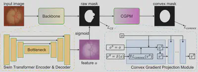
Figure 1: Overall framework. A Swin-Transformer encoder–decoder backbone produces feature $o$; a sigmoid yields the raw mask $u=\mathcal{S}(o)$. The Convex Gradient Projection Module (CGPM) is an unrolled gradient-descent block ($v^0 \rightarrow v^1 \rightarrow \cdots \rightarrow v^T$) that projects $u$ onto the quasi-concave manifold by descending the convex loss $\nabla\mathcal{L}_{\mathrm{convex}}$. The network is trained with cross-entropy $\mathcal{L}_{\mathrm{CE}}$ on the raw mask and the quasi-concavity loss $\mathcal{L}_{\mathrm{convex}}$ on the projected mask.
Animated Demo: Zero/First/Second-Order Convexification
The animation below visualizes the midpoint (zero-order), first-order gradient, and second-order Hessian convexification dynamics applied to a non-convex initial mask. All three orders progressively regularize the shape into a convex region, but with increasing levels of spatial smoothness.
Motivation
Convexity is a fundamental prior: many anatomical structures (optic disc/cup, blood vessels, organs) and man-made objects are convex or close-to-convex. Enforcing convexity suppresses holes, fragmented predictions, and irregular boundary artifacts, especially under noise, occlusion, and limited training data.
Existing approaches, however, have significant limitations:
- Discrete formulations (e.g. 1–0–1 collinear-triplet penalties, graph-cuts with convexity constraints, ILP/multicut decompositions) rely on combinatorial solvers and are hard to differentiate through.
- Level-set/curvature methods (non-negative curvature $\kappa\geq 0$, signed-distance Laplacian $\Delta\phi\geq 0$) certify convexity only at one chosen threshold (e.g. $\phi=0$) and are typically necessary but not sufficient.
- Recent deep shape priors still lack explicit, principled control over convexity at every confidence level.
D-Convexity resolves all three issues with a single functional view: the mask function $u$ itself should be quasi-concave.
Theory: Quasi-Concavity as a Unified Convex Prior
We formalize convexity threshold-freely as quasi-concavity of $u$:
$$ u \text{ is quasi-concave} \;\Longleftrightarrow\; \forall \gamma,\; S_\gamma=\{\mathbf{x}\mid u(\mathbf{x})\geq\gamma\}\ \text{is convex}. $$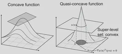
Figure 2: Concave vs. quasi-concave functions. A concave function (left) lies below every tangent plane — a strong property that most segmentation masks violate. A quasi-concave function (right) is the weaker, threshold-free notion D-Convexity uses: it only requires that every super-level set $S_\gamma$ be a convex region. At any boundary point $\mathbf{x}$, the supporting hyperplane is given by $\nabla u(\mathbf{x})^{\top}(\mathbf{y}-\mathbf{x})=0$ — this is the geometric content of our first-order condition.
By considering different smoothness assumptions on $u$, we derive three equivalent (or sufficient) characterizations:
Zero-order condition ($u\in C^0$)
$u$ is quasi-concave $\Longleftrightarrow$ for all $\mathbf{x},\mathbf{y}\in\Omega,\ \lambda\in[0,1]$:
$$u(\lambda\mathbf{x}+(1-\lambda)\mathbf{y}) \;\geq\; \min\{u(\mathbf{x}),u(\mathbf{y})\}.$$
A line segment joining two points above a level cannot dip below that level.
First-order condition ($u\in C^1$)
$u$ is quasi-concave $\Longleftrightarrow$ if $u(\mathbf{x})\geq u(\mathbf{y})$, then $\nabla u(\mathbf{y})^{\top}(\mathbf{x}-\mathbf{y})\geq 0.$
The gradient at every point defines a supporting hyperplane of the local super-level set.
Second-order condition ($u\in C^2$, sufficient)
If for all $\mathbf{x}\in\Omega$ with $\nabla u(\mathbf{x})\neq 0$ the Hessian $\nabla^2 u(\mathbf{x}) \prec 0$ (strict negative definite) on the tangent space $T_\mathbf{x}=\{\mathbf{d}\mid \nabla u(\mathbf{x})^{\top}\mathbf{d}=0\}$, then $u$ is quasi-concave.
For 2D images this has the compact convolutional form:
$$ Q_2(\mathbf{x}) \;=\; u_x^2\,u_{yy} \;-\; 2\,u_x u_y\,u_{xy} \;+\; u_y^2\,u_{xx} \;<\;0, $$a quadratic form in the image gradient that can be evaluated densely as a tiny fixed-kernel convolution — no thresholding required.
A unifying lens
Following Section 3.6 of the paper, D-Convexity recovers many existing convex priors as special cases, with each prior mapped to one of our zero-, first-, or second-order quasi-concavity conditions. The mapping below uses the exact references from the CVPR 2026 paper (arXiv:2605.19210v1):
Zero-order line-segment prior. Han, Kwon, Kim & Cho, Noise-Robust Pupil Center Detection with Shape-Prior Loss, IEEE Access 2020 require that for every $\mathbf{x},\mathbf{y}$ in the segmentation object, the line segment between them also lies inside it — this is exactly our zero-order condition (Theorem 1) applied over the image domain. Our formulation is more general because it applies to the continuous mask $u$ rather than a single thresholded region.
Half-disk / binary convexity characterization. The indicator-mask condition $(u-1)(b_r\ast(2u-1))\geq 0$ proposed in Liu, Tai & Luo, Convex Shape Prior for Deep Neural Convolution Network based Eye Fundus Images Segmentation, 2020, Luo, Tai & Wang, A New Binary Representation Method for Shape Convexity, Analysis & Applications 2022, and Luo, Chen, Xiao & Tai, A Binary Characterization Method for Shape Convexity, Applied Mathematical Modelling 2023 follows directly from our first-order supporting-hyperplane condition (Theorem 2): at a background pixel $\mathbf{y}$, Lemma 1 forces the foreground into the half-space $\nabla u(\mathbf{y})^{\top}(\mathbf{x}-\mathbf{y})\geq 0$, which intersected with a radius-$r$ disk gives $|B_r(\mathbf{y})\cap S|\leq \tfrac{1}{2}|B_r(\mathbf{y})|$.
Curvature priors $\kappa\geq 0$. Ukwatta et al., Efficient Convex Optimization-Based Curvature Dependent Contour Evolution, SPIE 2013 and Yang et al., A Level Set Method for Convexity Preserving Segmentation of Cardiac Left Ventricle, ICIP 2017 constrain non-negative curvature of level-set boundaries — corresponding to $Q_2(\mathbf{x})\leq 0$, the necessary but not sufficient weakening of our second-order condition $Q_2(\mathbf{x})<0$.
Signed-distance Laplacian priors $\|\nabla\phi\|=1$ with $\Delta\phi\geq 0$. Luo, Tai, Huo, Wang & Glowinski, Convex Shape Prior for Multi-Object Segmentation, ICCV 2019 and Yan, Tai, Liu & Huang, Convexity Shape Prior for Level Set-Based Image Segmentation, IEEE TIP 2020 impose non-negativity of the signed-distance Laplacian. With $\phi=-u$, the curvature identity $\kappa=-Q_2/\|\nabla u\|^3$ shows $\kappa\geq 0 \Leftrightarrow Q_2\leq 0$; D-Convexity’s strict $Q_2<0$ upgrades this into a sufficient convexity condition while remaining fully differentiable.
Related discrete convexity priors (discussed in Section 2 of the paper, and subsumed at the pixel-graph scale by our zero-order view) include 1–0–1 collinear-triple penalties (Gorelick, Veksler, Boykov & Nieuwenhuis, ECCV 2014 / TPAMI 2017), multicut / ILP convexity constraints (Royer, Richmond, Rother, Andres & Kainmüller, CVPR 2016), and relaxed star-type families (Veksler, ECCV 2008; Gulshan et al., CVPR 2010; Isack, Veksler, Sonka & Boykov, CVPR 2016).
So a single quasi-concavity principle subsumes discrete, half-disk, level-set, and curvature-based shape priors in one continuous, differentiable framework, with each prior corresponding to the smoothness order ($C^0$ / $C^1$ / $C^2$) at which it operates.
Loss Functions and CGPM
The first- and second-order conditions become local convolutional losses, evaluated densely over the image without any thresholding:
- First-order loss ($\mathcal{L}_{\text{1st}}$): penalize the positive part of the asymmetric pair inequality $\mathrm{ReLU}\big(\nabla u(\mathbf{y})^{\top}(\mathbf{y}-\mathbf{x})\big)$ over a small $r$-radius neighborhood $\mathbf{x}\in N_{\mathbf{y}}$.
- Second-order loss ($\mathcal{L}_{\text{2nd}}$): penalize the positive part of $Q_2(\mathbf{x})+\delta$ weighted by $\|\nabla u(\mathbf{x})\|$:
Both losses cost $\mathcal{O}(r^2|\Omega|)$ for the first-order and $\mathcal{O}(|\Omega|)$ for the second-order condition, are GPU-parallel, and have explicit closed-form gradients (see Appendix E of the paper).
Convex Gradient Projection Module (CGPM)
At inference time, the loss alone may not strictly enforce convexity. The CGPM solves a small proximal optimization on the network logits:
$$ u_p \in \arg\min_{v\in[0,1]} \tfrac{1}{2}\|v-u\|^2 + \lambda\cdot \mathcal{L}_{\text{convex}}(v), $$with $\mathcal{L}_{\text{convex}}\in\{\mathcal{L}_{\text{1st}},\mathcal{L}_{\text{2nd}}\}$. Implemented as an unrolled gradient-descent module on the logit space, CGPM is a drop-in projection layer compatible with any segmentation backbone (U-Net, nnU-Net, TransUNet, etc.):
from CGPM import SegModelWithCGPM

model = UNet2D().to(device)
model.load_state_dict(ckpt)
model.eval()

SegCGPM = SegModelWithCGPM(model, backprop_to_backbone=False)
cgpm_output = SegCGPM(images)
CGPM can be used in train mode (back-propagated into the backbone) or as a post-hoc projection (frozen backbone, projection only).
Experimental Results
We evaluate D-Convexity on four segmentation benchmarks spanning cardiac MRI (ACDC), iris segmentation (CASIA), and retinal optic-disc/cup segmentation (REFUGE, RIM-ONE-r3). To assess out-of-distribution generalization, models trained on REFUGE are evaluated directly on RIM-ONE-r3 without fine-tuning. Reported metrics are Dice ↑, IoU ↑, and Hausdorff Distance HD ↓.
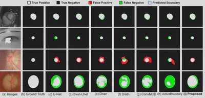
Qualitative comparison
Quantitative results
| Method | ACDC | CASIA | REFUGE | RIM-ONE-r3 | ||||||||
|---|---|---|---|---|---|---|---|---|---|---|---|---|
| Dice ↑ | IoU ↑ | HD ↓ | Dice ↑ | IoU ↑ | HD ↓ | Dice ↑ | IoU ↑ | HD ↓ | Dice ↑ | IoU ↑ | HD ↓ | |
| U-Net [28] | 89.52 | 81.02 | 28.04 | 94.65 | 89.84 | 2.549 | 84.66 | 73.71 | 11.07 | 76.48 | 61.92 | 20.57 |
| Swin-Unet [3] | 95.42 | 91.23 | 4.965 | 94.76 | 90.05 | 2.399 | 84.00 | 72.42 | 7.863 | 81.00 | 68.07 | 15.32 |
| DCAN [4] | 93.38 | 87.59 | 6.946 | 94.90 | 90.29 | 2.413 | 80.66 | 67.59 | 9.379 | 76.23 | 61.59 | 16.53 |
| DMTN [31] | 92.60 | 86.22 | 8.500 | 94.92 | 90.34 | 2.337 | 82.36 | 70.01 | 9.337 | 78.39 | 64.46 | 16.80 |
| ConvMCD [25] | 93.44 | 87.68 | 15.53 | 95.03 | 90.54 | 2.323 | 78.38 | 64.45 | 12.51 | 76.71 | 62.22 | 18.18 |
| Active Boundary [35] | 90.93 | 81.38 | 24.71 | 94.49 | 89.55 | 2.656 | 84.82 | 73.63 | 10.59 | 75.37 | 60.48 | 20.64 |
| Proposed (D-Convexity) | 95.46 | 91.31 | 4.702 | 94.71 | 89.94 | 2.288 | 88.61 | 79.54 | 5.859 | 83.09 | 71.08 | 12.59 |
Takeaways.
- Best overall on 3 of 4 datasets. D-Convexity is the top performer on ACDC, REFUGE, and RIM-ONE-r3 across all three metrics, and is best on Hausdorff Distance on CASIA. Dice/IoU on CASIA are essentially saturated for all methods (within 0.3% of each other).
- Largest gains on hard, shape-driven tasks. On REFUGE, D-Convexity improves Dice from 84.82 → 88.61 ( +3.79) and reduces HD from 7.863 → 5.859 ( −2.0) versus the strongest baseline, with similar gains on the ACDC cardiac task.
- Strong out-of-distribution generalization. When the REFUGE-trained model is applied directly to RIM-ONE-r3 (different acquisition device and population), D-Convexity still wins by +2.1 Dice and −2.7 HD over Swin-Unet — evidence that the convex shape prior acts as a robust, task-agnostic regularizer rather than overfitting to a particular dataset.
- Drop-in improvement. All gains are obtained with the same backbone segmentation network as the baselines, with CGPM as a plug-in module — no architectural changes are required.
Key Contributions
- Quasi-concavity as a unified convex prior. We formalize convexity of all super-level sets as quasi-concavity of the network output $u$, yielding a threshold-free, differentiable, image-domain constraint.
- Multi-order characterizations. Zero-, first-, and second-order conditions for $u\in C^0,C^1,C^2$, corresponding to different mask smoothness regimes.
- Compact convolutional losses. The first- and second-order conditions reduce to tiny fixed-kernel convolutions, allowing dense evaluation across the image at $\mathcal{O}(|\Omega|)$ cost.
- Convex Gradient Projection Module (CGPM). A plug-and-play unrolled-optimization module that strictly enforces convexity at inference time.
- Theoretical unification. Discrete 1–0–1 priors, half-disk convolution priors, and curvature / signed-distance Laplacian priors are all recovered as special cases or necessary weakenings of our framework.
- Empirical gains. Consistent convexity and shape-regularity improvements across multiple medical-imaging datasets (retinal fundus, cardiac MRI, iris, etc.), outperforming task-specific networks and prior shape-aware methods.
Quick Start
The reference implementation is available on GitHub: ShengzheC/D-Convexity.
For intuition on the convexification algorithm and the zero-order dynamics, start with the notebook:
Convexification_Algorithm.ipynb
The CGPM segmentation framework lives in CGPM.py, and the first- and second-order
losses in loss.py.
Resources
- Paper (arXiv): arXiv:2605.19210
- Code: github.com/ShengzheC/D-Convexity
- CVPR 2026 virtual poster: cvpr.thecvf.com/virtual/2026/poster/39174
- Venue: CVPR 2026 (Highlight, top 3%)
BibTeX
@InProceedings{Chen_2026_CVPR,
    author    = {Chen, Shengzhe and Yan, Hao},
    title     = {D-Convexity: A Unified Differentiable Convex Shape Prior via Quasi-Concavity for Data-driven Image Segmentation},
    booktitle = {Proceedings of the IEEE/CVF Conference on Computer Vision and Pattern Recognition (CVPR)},
    month     = {June},
    year      = {2026},
    pages     = {34755-34764}
}